Data Science Interview Questions (Part 2)

It is a table with 4 different combinations of predicted and actual values.

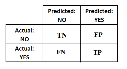
1. TP (True Positive) : The values were positive and predicted positive.
2. FP (False Positive) : The values were negative but falsely predicted as positive.
3. FN (False Negative) : The values were positive but falsely predicted as negative.
4. TN (True Negative) : The values were negative and were predicted negative.

The accuracy of a model (through a confusion matrix) is calculated using the given formula below.

What is Bagging and Boosting?

Bagging and boosting are two methods of implementing ensemble models.

Bagging

Bagging, short for bootstrap aggregating, is a powerful ensemble learning technique used to enhance the accuracy and robustness of machine learning models. In the bagging process, multiple models, known as learners, are constructed independently by creating random subsets from the training dataset. Each learner is then trained on its respective subset, introducing diversity in the model training process.

After training all the learners, their predictions are aggregated by taking the average of their individual outputs. This aggregation helps reduce variance and improve the overall predictive performance of the ensemble. However, it's important to note that increasing the size of the training set does not necessarily lead to better predictive power. Instead, it primarily aids in decreasing variance, fine-tuning predictions to align closely with the expected outcomes. Bagging is a valuable technique widely employed in machine learning to mitigate overfitting and produce more stable and reliable predictions across diverse applications.

Boosting

Boosting is a powerful ensemble learning technique that shares some similarities with bagging, such as sampling subsets with replacement to train multiple learners independently. However, the key difference lies in the way learners are trained and combined. In boosting, the first predictor is trained on the entire dataset, and subsequent predictors are trained based on the performance of the previous ones. This process is iterative, and each learner focuses on correcting the errors made by its predecessors.

Boosting begins by classifying the original dataset and assigning equal weights to each observation. If the first learner predicts classes incorrectly, higher weights are assigned to the misclassified observations. As the process iterates, subsequent learners prioritize those observations that were previously misclassified, leading to a refined and improved model.

Boosting has demonstrated superior predictive accuracy compared to bagging, as it actively adapts and corrects itself during training. However, it is important to be cautious about potential overfitting to the training data, as the iterative nature of boosting may result in excessively specialized models. Careful parameter tuning and setting limits on the number of models or accuracy are essential to mitigate overfitting and ensure generalizability to new data. Despite this concern, boosting remains a highly effective and widely used technique in machine learning, offering improved performance in many applications.

What are categorical variables?

A categorical variable is characterized by having a finite number of distinct values or categories. Such data attributes represent discrete and qualitative information, belonging to specific groups or classes.

For example, if individuals responded to a survey regarding their motorcycle ownership, the possible responses could be categorized into brands like "Yamaha," "Suzuki," and "Harley-Davidson." In this scenario, the data collected would be considered categorical, as it falls into distinct groups based on the available options. Categorical variables play a significant role in data analysis and are commonly encountered in various fields, including market research, social sciences, and customer surveys.

When to use ensemble learning?

When using decision trees, there is a trade-off between model complexity and the risk of overfitting. To accurately model complex datasets, decision trees may require many levels, but as the tree becomes deeper, it becomes more prone to overfitting the training data and may not generalize well to new data.

Ensemble learning techniques are employed to address overfitting and utilize the strengths of different classifiers to improve the model's stability and predictive power. Ensembles involve combining multiple predictive models to obtain a more robust and accurate prediction. The idea behind ensemble learning is that a group of weak predictors can outperform a single strong predictor. By training different models with diverse predictive outcomes and using the majority rule or weighted averaging as the final ensemble prediction, the overall result tends to be better than relying on a single model.

Ensemble methods, such as Random Forests, Gradient Boosting, and Bagging, have proven to be effective in enhancing the performance of machine learning models. They mitigate the risk of overfitting, increase generalization capabilities, and contribute to more accurate and reliable predictions. Ensembles have become a valuable tool in data science, particularly when dealing with complex and high-dimensional datasets.

What is the trade-off between accuracy and interpretability?

When constructing a predictive model, two critical criteria come into play: predictive accuracy and model interpretability. Predictive accuracy refers to the model's capability to make accurate predictions on new, unseen data. It is a measure of how well the model can identify and predict the occurrence of specific events or outcomes.

On the other hand, model interpretability pertains to the extent to which the model's inner workings are understandable to humans. An interpretable model provides insights into the relationships between input variables and the output, allowing users to comprehend why certain independent features influence the dependent attribute. This interpretability is valuable as it enables users to gain a deeper understanding of the factors driving the model's predictions and to extract meaningful insights from the data.

Both predictive accuracy and model interpretability are essential considerations when choosing or developing a predictive model. While high predictive accuracy is crucial for making reliable predictions, model interpretability is vital for gaining valuable insights and building trust in the model's decision-making process. Striking the right balance between these two criteria is often a challenge in the field of data science, as more complex models tend to offer higher predictive accuracy but might sacrifice interpretability. Data scientists must carefully weigh these factors based on the specific requirements and constraints of their applications.

What is a ROC Curve and How to Interpret It?

The ROC curve is a valuable tool in binary classification problems, aiding in the visualization of model performance. In binary classification, the model predicts whether a data point belongs to one of two potential classes, such as distinguishing between pedestrian and non-pedestrian input samples.

The Receiver Operating Characteristic (ROC) curve is commonly used as a representation of the trade-off between true positive rates (TPR) and false positive rates (FPR) at various thresholds. TPR, also known as sensitivity or recall, measures the proportion of true positive predictions out of all actual positive instances. On the other hand, FPR is the fraction of false positive predictions out of all actual negative instances and is equal to 1 - TPR. The ROC curve plots the TPR against the FPR, providing a visual depiction of the model's performance across different classification thresholds.

By examining the ROC curve, data scientists can assess how well the model distinguishes between the positive and negative classes. An ideal ROC curve would hug the top-left corner, indicating high sensitivity and low false positive rate, indicating that the model accurately classifies positive instances while minimizing misclassifications of negatives. In contrast, a diagonal ROC curve suggests that the model's performance is no better than random guessing, while a curve below the diagonal indicates poor performance. Analyzing the ROC curve helps data scientists choose an appropriate threshold that balances the true positive and false positive rates based on the specific requirements of their binary classification problem.

Explain PCA?

PCA, which stands for Principal Component Analysis, is a powerful feature transformation technique used in data analysis and machine learning. Its main objective is to rotate the original data dimensions and convert them into a new orthonormal feature space. In this new feature space, the principal components serve as the dimensions, and they are derived as linear combinations of the original feature dimensions.

The primary motivation behind using PCA is to address the "curse of dimensionality" problem that arises when dealing with large datasets with many features. As the number of features increases, the complexity of the data also grows, making it challenging to process and analyze effectively. PCA helps to overcome this issue by identifying the most significant patterns and relationships among the original features and transforming the data into a lower-dimensional space.

Differences between supervised and unsupervised learning?

Supervised learning is a type of algorithm that involves providing a known set of input data along with corresponding known responses or outputs. The goal is to train a model that can make accurate predictions for new, unseen data. The input data, denoted as "x," is paired with the expected outcomes or responses, denoted as "y," which are often referred to as the "class" or "label" of the corresponding input.

Supervised learning is used for two main types of problems: Classification and Regression. In classification, the model is trained to categorize input data into specific classes or categories. For example, it can be used to predict whether an email is spam or not spam based on its content. In regression, the model is trained to predict a continuous value, such as predicting the price of a house based on its features.

On the other hand, unsupervised learning does not have known categories or labels for the input data. Instead, it aims to find patterns, correlations, or structures in the data without any external inputs other than the raw data itself. Unsupervised learning can be used for two main types of problems: Clustering and Association. In clustering, the algorithm groups similar data points together to form clusters, based on the similarity of their features. In association, the algorithm identifies relationships or associations between different variables in the dataset.

Explain univariate, bivariate, and multivariate analyses.

1. Univariate analyses only one variable at a time.
2. Bivariate analyses compare two variables.
3. Multivariate analyses compare more than two variables.