Logistic Regression in Machine Learning
Logistic regression is a statistical method used for binary classification tasks. It predicts the probability of a binary outcome (e.g., yes or no, pass or fail, spam or not spam) based on a set of independent variables. Logistic regression is a supervised learning algorithm, meaning it learns from labeled data to make predictions on unlabeled data.
How does Logistic Regression work?
Logistic Regression utilizes the concept of logistic function, which transforms a real-valued input into a probability between 0 and 1. The logistic function maps the input to a probability, representing the likelihood of the positive class (e.g., spam) occurring.
The logistic regression model can be represented mathematically as:
- y: Predicted probability of the positive class
- σ: Logistic function (sigmoid function)
- w: Weights of the model
- x: Input vector of features
- b: Bias term
The goal of logistic regression is to find the optimal values of the weights (w) and bias (b) that minimize the error between the predicted probabilities and the true labels. This optimization process is typically performed using an iterative algorithm,
Fitting the Logistic Function
The parameters of the logistic function (b) are estimated using a technique called maximum likelihood estimation. Maximum likelihood estimation aims to find the values of the parameters that maximize the probability of observing the training data given the model.
Classification
Once the parameters of the logistic function have been estimated, the model can be used to classify new data points. For a new data point, the model calculates the probability of the positive class. If the probability is greater than or equal to 0.5, the data point is classified as the positive class. Otherwise, it is classified as the negative class.
Logistic Regression example
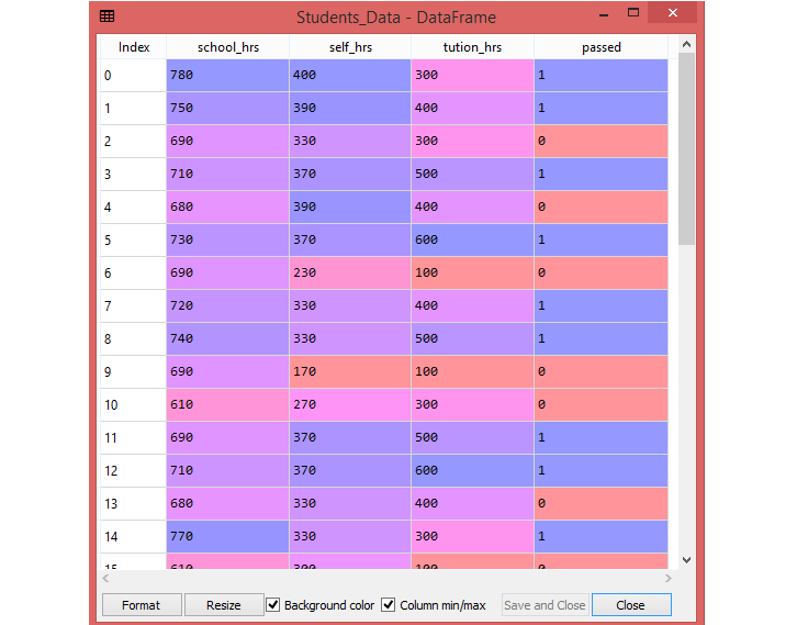
The students_data.csv dataset has three features—namely, school_hrs, self_hrs and tution_hrs. The school_hrs indicates how many hours per year the student studies at school, self_hrs indicates how many hours per year the student studies at home, and tution_hrs indicates how many hours per year the student is taking private tuition classes.
Apart from these three features, there is one label in the dataset named "passed ". This label has two values—either 1 or 0. The value of 1 indicates pass and a value of 0 indicates fail.
The file is meant for testing purposes only, you can download it from here: students_data.csv .
Here, you can build a Logistic Regression using:
- The dependent variable "passed" represents whether a student passed or not.
- The 3 independent variables are the school_hrs, self_hrs and tution_hrs.
To access the complete source code for the Logistic Regression example with explanation, click on the following link: Logistic Regression Example
Key Concepts of Logistic Regression
Binary Classification: The Core of Logistic Regression
Logistic regression is specifically designed for binary classification tasks, where the target variable or outcome has only two possible values. These values are often represented as labels such as "yes" or "no," "pass" or "fail," or "spam" or "not spam." The goal of logistic regression is to predict the probability of the positive outcome based on the values of the independent variables or features.
Logistic Function: Squishing Inputs into Probabilities
At the heart of logistic regression lies the logistic function, also known as the sigmoid function. This function acts as a transformation mechanism, taking any real-valued input and mapping it to a value between 0 and 1. The logistic function effectively squashes the input values within the range of 0 and 1, representing the probability of the positive outcome.
Decision Boundary: Separating Classes
The logistic regression model constructs a decision boundary, which is a line or curve that divides the data points into two regions based on the predicted probabilities. The decision boundary represents the threshold at which the model predicts the positive outcome. Data points on one side of the boundary are classified as positive, while those on the other side are classified as negative.
Log-Odds Ratio: Unveiling Feature Importance
The coefficients obtained from the logistic regression model hold valuable information about the importance of each independent variable in influencing the probability of the positive outcome. These coefficients represent the log-odds ratio, which measures the change in the log-odds of the positive outcome for a one-unit change in the corresponding independent variable. A positive coefficient indicates that an increase in the independent variable increases the odds of the positive outcome, while a negative coefficient suggests the opposite.
Limitations of Logistic Regression
Binary Classification Limitation: Constrained to Two Outcomes
Logistic regression is inherently designed for binary classification tasks, limiting its applicability to problems where the target variable or outcome can only take on two distinct values. This restriction can be a significant drawback when dealing with multi-class classification problems, where the target variable can have more than two possible categories. For instance, logistic regression cannot be used directly to classify fruits into multiple categories like apples, oranges, and bananas.
Linearity Assumption: Straight-Line Relationships Only
Logistic regression makes a fundamental assumption that the relationship between the log-odds of the positive outcome and the independent variables is linear. This means that the model assumes a straight-line relationship between the features and the probability of the positive outcome. If the true relationship is nonlinear, logistic regression may struggle to capture the underlying patterns, leading to inaccurate predictions.
Overfitting Risk: Memorizing Training Data
Logistic regression is prone to overfitting, especially when dealing with a large number of features or when the training data is limited. Overfitting occurs when the model learns the training data too well, including the noise and random fluctuations, and fails to generalize effectively to unseen data. This results in poor performance on new data points, as the model has not learned the true underlying relationships.
Addressing Limitations: Techniques and Alternatives
To address these limitations, several strategies can be employed:
- Multi-class Classification Extensions: For multi-class classification problems, extensions of logistic regression, such as multinomial logistic regression or one-versus-all logistic regression, can be used to transform the problem into multiple binary classification tasks.
- Nonlinear Transformations: If the true relationship is nonlinear, features can be transformed using techniques like polynomial transformations or kernel functions to capture nonlinear patterns.
- Regularization Techniques: Regularization methods, such as L1 or L2 regularization, can be applied to penalize large coefficients and reduce the model's complexity, mitigating overfitting.
- Alternative Models: For nonlinear relationships or multi-class classification, alternative models like support vector machines, decision trees, or neural networks may be more suitable.
Conclusion
Logistic regression is a fundamental and versatile machine learning algorithm for binary classification tasks. Its simplicity, interpretability, and robustness make it a valuable tool for a wide range of applications. However, it's essential to carefully consider the assumptions of logistic regression and address potential limitations to ensure reliable and valid results.