Linear Regression for Machine Learning

The goal of linear regression is to find the values of ß0 and ß1 that minimize the sum of squared errors (SSE). The SSE is the sum of the squares of the differences between the predicted values of y and the actual values of y.

There are several methods for estimating the coefficients, but the most common method is ordinary least squares (OLS) regression. OLS regression is a statistical method that finds the values of ß0 and ß1 that minimize the SSE.

Types of Linear Regression

Linear regression is a versatile supervised learning algorithm used for predicting a continuous outcome based on one or more predictor variables. It comes in two primary types: Single Linear Regression and Multiple Linear Regression.

Simple Linear Regression

In simple linear regression, we have only one independent variable. The equation for simple linear regression is:

where:

1. y is the dependent variable
2. x is the independent variable
3. m is the slope of the line
4. b is the y-intercept of the line

The slope m represents the change in the dependent variable y for a one-unit change in the independent variable x. The y-intercept b represents the value of the dependent variable y when the independent variable x is zero.

Simple Linear Regression Example:

The following Machine Learning example create a dataset that has two variables: Stock_Value (dependent variable, y) and Interest_Rate e (Independent variable, x). The purpose of this example is:

1. Find out if there is any correlation between these two (x,y) variables.
2. Find the best fit line for the dataset.
3. How the output variable is changing by changing the input variable.

To implement the Simple Linear Regression model in Machine Learning, you need to follow these steps:

1. Process the data
2. Split your dataset to train and test
3. Fitting the data to the Training Set
4. Prediction of test set result
5. Final Result
6. Visualizing Results

To access the complete source code for the Simple Linear Regression example with explanation, click on the following link: Simple Linear Regression example.

Multiple Linear Regression

In multiple linear regression, we have two or more independent variables. The equation for multiple linear regression is:

where:

1. y is the dependent variable
2. x1, x2, ..., xP are the independent variables
3. b0, b1, ..., bp are the coefficients of the independent variables

The coefficients b1, b2, ..., bp represent the change in the dependent variable y for a one-unit change in the corresponding independent variable x1, x2, ..., xp, when the other independent variables are held constant.

Multiple linear regression Example:

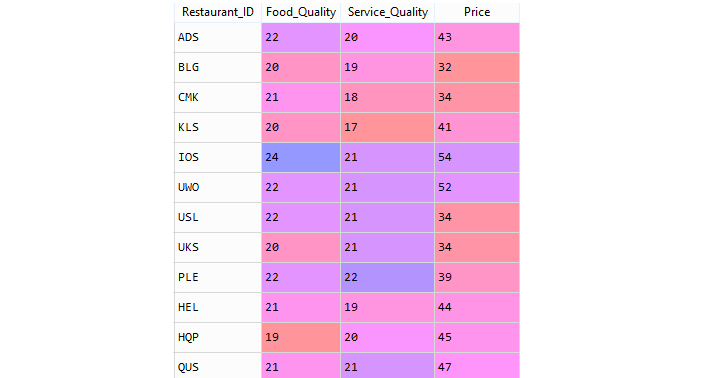
Consider the Restaurant data set: restaurants.csv . A restaurant guide collects several variables from a group of restaurants in a city. The description of the variables is given below:

Field	Description
Restaurant_ID	Restaurant Code
Food_Quality	Measure of Quality Food in points
Service_Quality	Measure of quality of Service in points
Price	Price of meal

Restaurant data sample,

To access the complete source code for the Multiple linear regression example with explanation, click on the following link: Multiple linear regression example.

Assumptions Underpinning Linear Regression Integrity

Linearity: Relationship between variables is linear

This assumption posits that the relationship between the independent and dependent variables can be adequately represented by a straight line. In other words, a change in the independent variable should correspond to a constant change in the dependent variable. Linear regression models assume this linearity to make predictions, and if the relationship is non-linear, the model may not accurately capture the underlying patterns in the data.

Independence: Residuals are independent

Independence of residuals means that the error terms (residuals) for different data points are not correlated. In simpler terms, the error in predicting one data point should not provide information about the error in predicting another. If there is correlation among residuals, it suggests that the model is not capturing some underlying pattern in the data, and the results may be unreliable. Independence is a crucial assumption for the statistical validity of parameter estimates and hypothesis testing in linear regression.

Homoscedasticity: Residuals have constant variance

Homoscedasticity refers to the assumption that the variance of the residuals should be constant across all levels of the independent variables. In practical terms, it means that the spread of the residuals should be consistent as you move along the range of predicted values. If the variance is not constant (heteroscedasticity), the model might be giving too much weight to certain data points, leading to unreliable predictions. Detecting and addressing heteroscedasticity is crucial for improving the precision of the model's predictions.

Normality: Residuals are normally distributed

The assumption of normality pertains to the distribution of the residuals, not necessarily the distribution of the independent and dependent variables. Ideally, the residuals should follow a normal distribution. Normality is crucial for making valid statistical inferences and constructing reliable confidence intervals and hypothesis tests. However, linear regression is often robust to departures from normality, especially with large sample sizes, thanks to the Central Limit Theorem. Still, extreme departures from normality might signal issues with the model or the data that should be investigated.

Key Concepts in Linear Regression

Linear regression is a fundamental machine learning algorithm that establishes a linear relationship between a dependent variable (target) and one or more independent variables (features). It is widely used for predictive modeling, trend analysis, and understanding causal relationships between variables. To effectively utilize linear regression, it's crucial to grasp the following key concepts:

Dependent Variable

The dependent variable, also known as the target variable or response variable, is the variable we are trying to predict or explain. It represents the outcome or measure of interest in the analysis. In simple linear regression, there is only one dependent variable, while in multiple linear regression, there can be multiple dependent variables.

Independent Variables

Independent variables, also known as predictor variables or explanatory variables, are the factors that influence or affect the dependent variable. They are the inputs that the model uses to make predictions about the dependent variable. In simple linear regression, there is only one independent variable, while in multiple linear regression, there can be multiple independent variables.

Coefficient Interpretation

The coefficients in a linear regression model represent the magnitude of change in the dependent variable for a one-unit change in the corresponding independent variable, assuming all other independent variables remain constant. Coefficients provide insights into the strength and direction of the relationship between the independent and dependent variables. A positive coefficient indicates a positive correlation, while a negative coefficient indicates a negative correlation.

Cost Function

The cost function, also known as the loss function, measures the error between the predicted values by the linear regression model and the actual values of the dependent variable. It serves as a performance metric for the model, indicating how well it fits the data. Common cost functions include mean squared error (MSE) and mean absolute error (MAE).

Gradient Descent

Gradient descent is an optimization algorithm used to minimize the cost function and find the best fitting line for the linear regression model. It iteratively updates the coefficients of the model by moving in the direction of the steepest descent of the cost function. This process continues until the cost function reaches a minimum, resulting in the optimal set of coefficients for the model.

These key concepts provide a foundation for understanding linear regression and its applications in various domains.

Applications of Linear Regression

Linear regression is a versatile algorithm that can be used for a wide variety of applications, including:

1. Predictive modeling: Predicting future values of a dependent variable based on past data.
2. Trend analysis: Identifying trends and patterns in data over time.
3. Causal inference: Understanding the causal relationship between variables.

Conclusion

Linear regression is a supervised machine learning algorithm that predicts a continuous outcome based on one or more predictor variables by establishing a linear relationship. It comes in two types: Single Linear Regression for one predictor variable and Multiple Linear Regression for multiple predictors, both aiming to minimize the difference between predicted and actual values through the optimization of coefficients.