Polynomial Regression in Machine Learning

The degree of the polynomial is a crucial parameter in polynomial regression. Choosing too low a degree may not capture the nonlinearity in the data, while choosing too high a degree may lead to overfitting. Overfitting occurs when the model memorizes the training data too well and fails to generalize to new data.

There are several methods for choosing the appropriate degree of the polynomial. One common method is to use trial and error, fitting polynomial models of different degrees and evaluating their performance using a cross-validation set. Another method is to use information criteria, such as the Akaike information criterion (AIC) or the Bayesian information criterion (BIC). These criteria balance the goodness of fit of the model with its complexity.

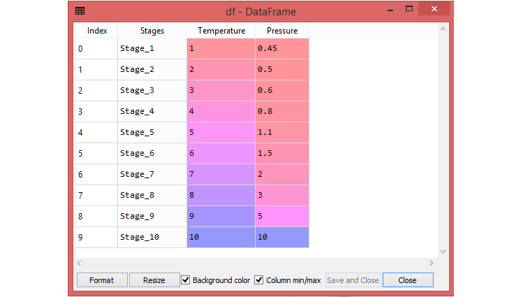
Polynomial Regression example

Here, some data of Pressure and Temperature related to each stages. So, using Polynomial Regression , check whether the data is showing the True or False in each stage. By checking the data available, found that there is a non-linear relationship between the Pressure and the Temperature. So, the goal is to build a Truth detector regression model using Polynomial Regression.

To access the complete source code for the Polynomial Regression example with explanation, click on the following link: Polynomial Regression Example

Key Concepts of Polynomial Regression

Nonlinear Relationships in Polynomial Regression

Linear regression, a fundamental statistical method, assumes a straight-line relationship between the dependent variable (target variable) and the independent variables (predictor variables). However, in many real-world scenarios, the relationship between variables may not be linear. This is where polynomial regression comes into play. Polynomial regression is a type of regression analysis that allows for modeling nonlinear relationships between variables. It utilizes polynomial functions, which are mathematical expressions that involve variables raised to different powers, to capture the curvature or non-linearity in the relationship between variables.

Polynomial Degree and Model Complexity

The degree of the polynomial function determines the complexity of the relationship that can be modeled. A higher degree polynomial can capture more intricate curves and non-linear patterns in the data. For instance, a quadratic polynomial (degree 2) can capture U-shaped or inverted U-shaped curves, while a cubic polynomial (degree 3) can model S-shaped curves. However, as the polynomial degree increases, the model becomes more complex and susceptible to overfitting.

Model Selection and Overfitting

Overfitting occurs when the model fits the training data too well, capturing even the noise and random fluctuations in the data. This leads to poor performance on unseen data, as the model is unable to generalize to new data points. To avoid overfitting, it is crucial to select the appropriate degree of the polynomial. Techniques like cross-validation can help determine the optimal polynomial degree by evaluating the model's performance on multiple subsets of the data.

Interpretability and Higher-Order Coefficients

While polynomial regression can capture complex relationships, interpreting the higher-order coefficients becomes increasingly challenging as the polynomial degree increases. For example, in a quadratic polynomial, the coefficient of the squared term represents the rate of change of the slope. In higher-degree polynomials, these interpretations become more intricate and may not have direct physical or intuitive meaning.

Balancing Model Complexity and Generalizability

The key to successful polynomial regression lies in balancing model complexity and generalizability. A higher-degree polynomial may capture more complex relationships but is more prone to overfitting. On the other hand, a lower-degree polynomial may not capture the true complexity of the relationship, leading to underfitting. Techniques like cross-validation and regularization can help achieve this balance, ensuring that the model generalizes well to unseen data while capturing the underlying relationship between variables.

Applications of Polynomial Regression

Polynomial regression is useful for modeling a wide range of nonlinear relationships, including:

1. Predicting sales trends: Predicting sales figures based on time or promotional efforts.
2. Modeling population growth: Estimating population growth over time, accounting for non-linear demographic factors.
3. Analyzing engineering data: Predicting material properties or system behavior based on non-linear relationships between variables.

Limitations of Polynomial Regression

Overfitting Risk in Polynomial Regression

Polynomial regression is particularly susceptible to overfitting, especially when high-degree polynomials are employed. Overfitting occurs when a model fits the training data too well, even capturing the noise and random fluctuations within the data. This results in poor performance on unseen data, as the model fails to generalize effectively to new data points. The increased flexibility of higher-degree polynomials, while allowing for more complex relationship modeling, also increases the risk of overfitting. The model may learn the intricacies of the training data, including the noise, rather than the underlying true relationship between variables.

Interpretability Challenges with Higher-Order Coefficients

As the degree of the polynomial function increases, interpreting the higher-order coefficients becomes increasingly challenging. While the coefficients in a linear regression model can be directly interpreted as the change in the dependent variable for a one-unit change in the corresponding independent variable, this straightforward interpretation becomes less clear for higher-degree polynomials. For instance, in a quadratic polynomial, the coefficient of the squared term represents the rate of change of the slope. In higher-degree polynomials, these interpretations become more intricate and may not have direct physical or intuitive meaning.

Model Complexity and Computational Demands

Polynomial regression models become more complex as the polynomial degree increases. This increased complexity leads to higher computational demands, especially during the training process. The number of parameters to estimate increases with the polynomial degree, requiring more computational resources to optimize the model parameters. This can be particularly challenging for large datasets or high-dimensional data.

Strategies for Mitigating Limitations

To mitigate the limitations of polynomial regression, several strategies can be employed:

Model Selection Techniques

Utilize techniques like cross-validation to select the optimal polynomial degree that balances model complexity and generalizability. Cross-validation involves evaluating the model's performance on multiple subsets of the data, providing insights into its generalizability to unseen data.

Regularization Techniques

Implement regularization techniques, such as ridge regression or lasso regression, to penalize higher-order coefficients and reduce the model's complexity. Regularization helps control the influence of higher-degree terms, mitigating overfitting without compromising the ability to capture complex relationships.

Data Preprocessing

Employ data preprocessing techniques, such as normalization or standardization, to scale the features to a similar range. This can help prevent numerical instability during the optimization process and improve the overall performance of the model.

Feature Engineering

Consider feature engineering techniques to create new features that capture more complex relationships between the original variables. This can involve transformations, interactions, or domain-specific knowledge to enhance the model's ability to capture nonlinear relationships.

Alternative Models

Explore alternative models, such as kernel regression or decision trees, which may be better suited for specific types of nonlinear relationships. These models can provide more flexibility in capturing complex patterns without the same susceptibility to overfitting as polynomial regression.

Conclusion

Polynomial regression is a powerful tool for modeling nonlinear relationships between variables and making predictions based on those relationships. Its flexibility, adaptability, and predictive power make it valuable for a wide range of applications. However, it's crucial to carefully select the polynomial degree to balance model complexity and generalizability, avoiding overfitting and ensuring interpretability.