Polynomial Regression | Python Machine Learning
Regression is a powerful statistical method used to establish relationships between the independent variables (inputs used for prediction) and the dependent variable (the variable being predicted) to make outcome predictions.
When the data points do not follow a linear pattern, Polynomial Regression is a suitable alternative. It allows for modeling relationships that are not linear by using higher-order polynomials, enabling the prediction of outcomes with more complex curves. This flexibility makes Polynomial Regression a valuable tool in situations where linear relationships do not adequately capture the underlying data patterns.
The equation of the Polynomial Regression having an nth degree can be written as:

Polynomial Regression example | Python
Here, some data of Pressure and Temperature related to each stages. So, using Polynomial Regression , check whether the data is showing the True or False in each stage. By checking the data available, found that there is a non-linear relationship between the Pressure and the Temperature. So, the goal is to build a Truth detector regression model using Polynomial Regression. Below are the steps to build such a model.
Import the Python libraries
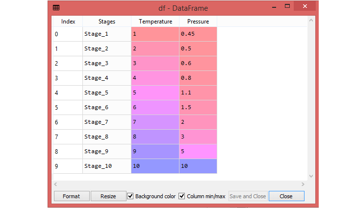
Define dataset
Extracted the dependent(y) and independent variable(x) from the dataset.
The dataset contains three columns (Stages, Temperature, and Pressure), but, here consider only two columns (Temperature and Pressure). In the following Polynomial Regression model , predict the output for Temperature 6.5 somewhere between stage_6 and stage_7.
In building Polynomial Regression, it is better to take the Linear regression model as reference and compare both the output.
Building the Linear regression model
Above code create a Simple Linear model using linear_regs object of LinearRegression class and fitted it to the dataset variables (x and y).
Building the Polynomial regression model
Above code used polynomial_regs.fit_transform(x) , because first it convert your feature matrix into polynomial feature matrix, and then fitting it to the Polynomial regression model. The argument (degree= 2) depends on your choice. You can choose it according to our Polynomial features .
After executing the code, you will get another matrix x_poly, which you can be seen under the Spyder variable explorer:
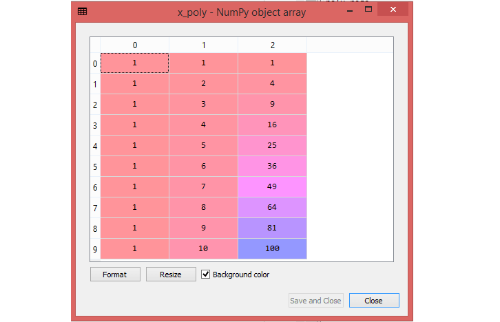
Next step is to use another LinearRegression object , namely linear_reg_2, to fit your x_poly vector to the linear model.
Linear regression Plot
Visualize the result for Linear regression model as you did in Simple Linear Regression.
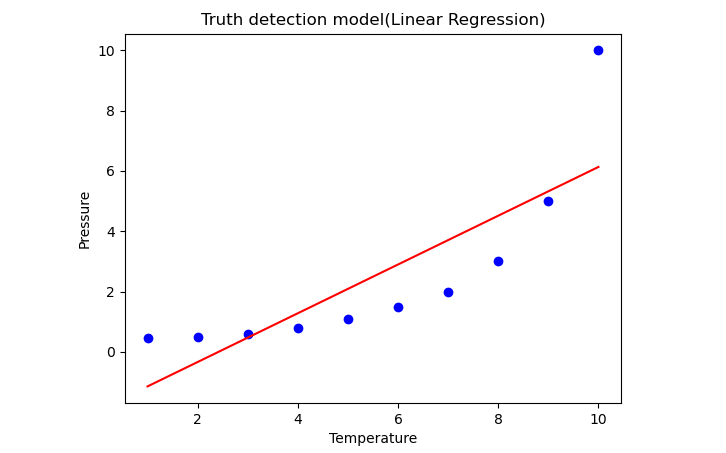
Here, you can see that the regression line is so far from the datasets. Actual values in blue data points and Predictions are in a red straight line. If you consider this output to predict the value of Temperature, in some cases which is far away from the real value.
So, you need a curved model to fit the dataset other than a straight line.
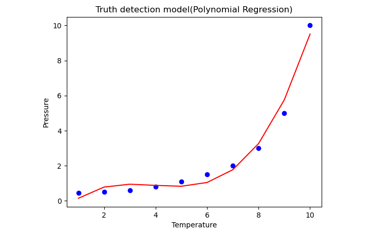
Polynomial Regression Plot
Here, you have taken linear_reg_2.predict(poly_regs.fit_transform(x), instead of x_poly, because you want a Linear regressor object to predict the polynomial features matrix .
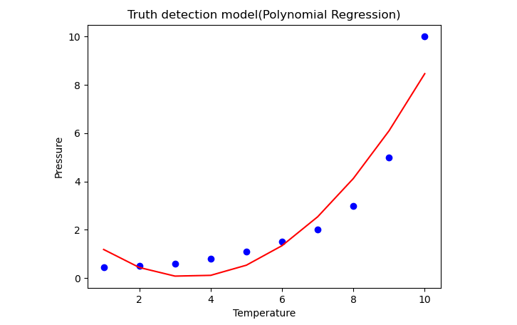
In the above image you can see the predictions are close to the real values. The above plot will vary as you will change the degree.
Change degree= 3
Above image will give you a more accurate plot when you change the degree=3.
Change degree= 4
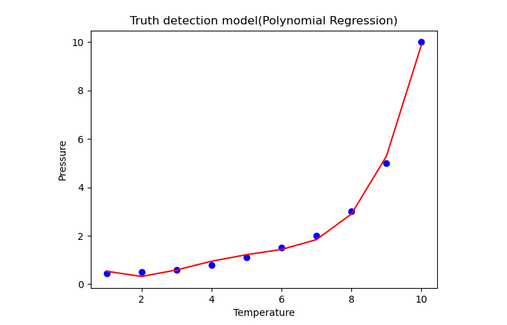
Above image will give you a most accurate plot. So, you will get more accurate results by increasing the degree of Polynomial.
Predicting the final result
Next step is to predict the final output using the models to see whether the data is true or false.
Linear Regression model
Here use the predict() method and will pass the value 6.5.
Polynomial Regression model
Here also use the predict() method and will pass the value 6.5.
Above code confirms that the predicted output for the Polynomial Regression is [1.58862453], which is much closer to real value.
Full Source | PythonConclusion
Polynomial Regression is a type of regression analysis that extends the concept of linear regression to model non-linear relationships between independent and dependent variables. It utilizes higher-order polynomial functions to capture more complex patterns in the data, making it a valuable technique when linear regression is insufficient to represent the underlying relationship between variables.