Random Forests Classifiers | Python
Random Forest is a powerful ensemble learning algorithm that consists of multiple decision trees. Each decision tree makes predictions with a certain level of accuracy, but when combined in a forest, they create a more robust and accurate prediction model. The aggregation of multiple trees helps prevent overfitting and improves the overall accuracy of the Random Forest algorithm, making it a popular choice for various classification and regression tasks in supervised learning.
In the Random Forest algorithm, the "forest" is an ensemble of decision trees that are trained using the "bagging" method. Bagging stands for Bootstrap Aggregating, and it involves training each decision tree on a random subset of the original training data, allowing for diversity and reducing the variance in the predictions. The combination of multiple decision trees through bagging produces a more robust and accurate prediction model, making Random Forest a powerful and widely used supervised learning algorithm.
Ensemble methods
The primary goal of ensemble algorithms is to combine the predictions of multiple base estimators, typically generated using the same learning algorithm, to enhance the overall performance and robustness over using a single estimator. By aggregating the predictions from multiple models, ensemble algorithms reduce the risk of overfitting and improve the accuracy and generalization of the final prediction, making them powerful tools in machine learning for both classification and regression tasks.
Bagging methods
Bootstrap Aggregation, also known as Bagging, is an ensemble meta-algorithm that aims to improve the accuracy and robustness of predictions by combining the outputs of multiple base learners. The idea behind bagging is to train several base models, each on a randomly sampled subset of the training data, and then aggregate their predictions to produce a more accurate and reliable overall output. Bagging is widely used in various machine learning algorithms, including Random Forests, to reduce variance, prevent overfitting, and enhance the performance of the final prediction model.
Hyper-parameters
Hyperparameters in the Random Forest model are settings that are not learned from the training data but need to be set by the user before training the model. These hyperparameters are crucial for controlling the behavior of the Random Forest algorithm. They can be tuned to increase the predictive power of the model by finding the best configuration for the given problem, or they can be adjusted to make the model faster and more efficient. Properly tuning the hyperparameters can significantly impact the performance and efficiency of the Random Forest model.
n_estimators
In the Random Forest algorithm, the n_estimators hyperparameter determines the number of decision trees to be used in the ensemble. Increasing the number of estimators (trees) generally improves the performance of the Random Forest by reducing overfitting and increasing the accuracy of the predictions. However, a higher number of estimators may also increase the computational cost and training time of the model. Finding the optimal value for n_estimators through cross-validation and performance evaluation is essential to strike the right balance between accuracy and efficiency in the Random Forest model.
max_features
The max_features hyperparameter controls the maximum number of features that the algorithm considers when looking for the best split at each node of the decision tree. By limiting the number of features, Random Forest reduces the randomness and prevents overfitting, making the model more robust and less sensitive to noise in the data. Setting max_features to a lower value can improve the performance and generalization of the model by promoting diversity among the individual decision trees in the ensemble.
n_jobs
The n_jobs parameter allows you to specify the number of processor cores that the algorithm is allowed to utilize during training and prediction. By setting n_jobs to a higher value, you can make use of multiple processor cores, which can significantly speed up the training process, especially when dealing with large datasets or complex models. It's a useful parameter to optimize the performance of the Random Forest algorithm, especially on systems with multi-core processors.
random_state
The random_state parameter in scikit-learn's Random Forest (and other algorithms) is used to set a seed for the random number generator. This ensures that the train-test splits and other random operations within the algorithm are always reproducible and deterministic across different runs. By setting the random_state to a fixed value, you can obtain consistent and predictable results, which is essential for debugging, experimentation, and making comparisons between different runs or models.
Python implementation of the Random Forest algorithm
The final outcome is determined by aggregating the predictions of individual decision trees. For regression tasks, the algorithm takes the average or mean of the predictions from all the trees to make the final prediction. For classification tasks, it uses majority voting to determine the class label with the highest frequency among the predictions.
Increasing the number of trees in the Random Forest ensemble generally leads to a more precise and accurate outcome. As the number of trees grows, the variance and overfitting reduce, resulting in a more robust and reliable model. However, it is essential to find the right balance between increasing the number of trees and the computational resources required, as a very large number of trees may also lead to increased training time and memory usage.
About the Dataset
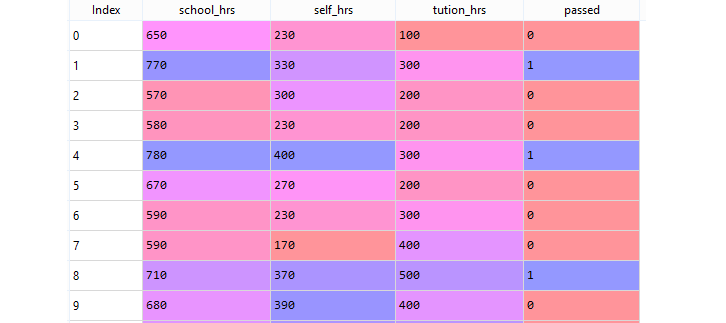
The "study_hours.csv" dataset contains information on students with four features: "school_hrs," which represents the number of hours per year the student studies at school, "self_hrs," indicating the number of hours per year the student studies at home, "tution_hrs," which represents the number of hours per year the student takes private tuition classes, and "passed," which indicates whether the student passed (1) or failed (0). This dataset can be used for various machine learning tasks, such as regression or classification, to predict the likelihood of a student passing based on their study hours at school, at home, and private tuition classes.
The "passed" variable in the "study_hours.csv" dataset serves as the dependent variable or the target variable. It is a binary categorical variable with two values: 1 indicates a pass, and 0 indicates a fail. The objective of using this dataset for machine learning would be to predict the student's outcome (pass or fail) based on the independent variables "school_hrs," "self_hrs," and "tution_hrs." This is a typical binary classification problem, where the model will try to learn the relationship between study hours and passing outcome to make predictions for new students.
The file is meant for testing purposes only, download it from here: study_hours.csv .
Sample Data from study_hours.csv :
Import Python Packages
Create the DataFrame
Data Pre-Processing
The X variable contains the threee columns (school_hrs, self_hrs, tution_hrs) of the dataset while y contains the target column "passed".
Apply train_test_split
Above code, set the test size to 0.25 , and therefore the model testing will be based on 25% of the dataset, while the model training will be based on 75% of the dataset.
The random_state parameter in scikit-learn's train_test_split function is used to set a seed for the random number generator that determines how the data is split into training and testing sets. If you do not specify a random_state, a new random value will be generated each time you run your code, resulting in different train and test datasets in each run.
However, if you set a fixed value for random_state, such as random_state = 0, the random number generator will produce the same sequence of random numbers every time you execute your code. As a result, the train and test datasets will be the same across different runs, which is useful for reproducibility and consistent evaluation of the model's performance during experimentation and development.
Building a Random Forest Model
n_estimators is used to control the number of trees to be used in the process.
Making Predictions With Random Forest Model
Once your Random Forest Model training is complete, its time to predict the data using the created model. So, you can store the predicted values in the y_pred variable.
Accuracy and Confusion Matrix
Once the prediction is over, the next step is to print the accuracy and plot the confusion matrix .
Confusion Matrix
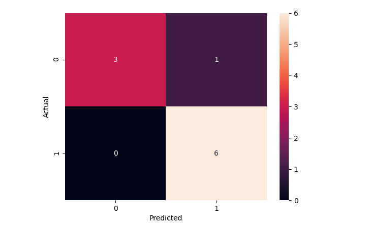
You can also derive the Accuracy from the above Confusion Matrix :
Accuracy = (True Positives + True Negatives)/(Sum of all values on the matrix)Accuracy = (6+3)/(3+1+0+6)
Accuracy = (9)/(10)
Accuracy = 0.9 * 100 = 90 % Full Source | Python
Checking the Prediction
Recall that your original dataset ("study_hours.csv") had 40 observations . Since you set the test size to 0.25 , then the Confusion Matrix displayed the results for a total of 10 records (=40*0.25). These are the 10 test records:
The prediction was also made for those 10 records on target field "passed" represents whether a student passed or not(either 1 or 0. The value of 1 indicates pass and a value of 0 indicates fail).
From the following table you can confirm that you got the correct results 9 out of 10 .
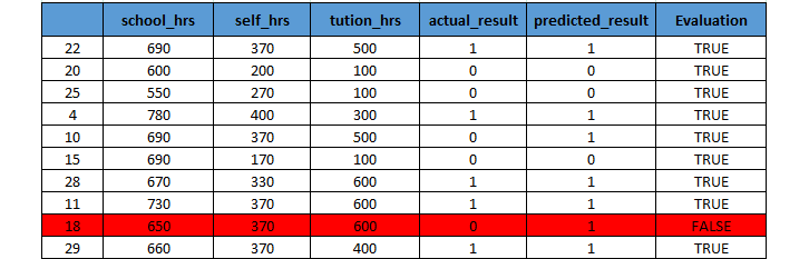
From the above table, you can confirm that the result matching with the accuracy level of 90% .
Conclusion
Random Forest Classifiers are an ensemble learning method that combines multiple decision trees to make more accurate and robust predictions. By aggregating the predictions of individual trees through voting or averaging, Random Forests can handle both classification and regression tasks effectively. They are widely used in machine learning due to their ability to reduce overfitting, handle complex datasets, and provide high accuracy and generalization.