Simple Linear Regression | Python

With Simple Linear Regression model your data as follows:

This is a line where y(pred) is the output variable you want to predict, x is the input variable and B0 and B1 are coefficients that you need to estimate that move the line around.

Simple Linear Regression example

The following Machine Learning example create a dataset that has two variables: Stock_Value (dependent variable, y) and Interest_Rate e (Independent variable, x). The purpose of this example is:

1. Find out if there is any correlation between these two (x,y) variables.
2. Find the best fit line for the dataset.
3. How the output variable is changing by changing the input variable.

To implement the Simple Linear Regression model in Machine Learning, you need to follow these steps:

1. Process the data
2. Split your dataset to train and test
3. Fitting the data to the Training Set
4. Prediction of test set result
5. Final Result
6. Visualizing Results

Process the data

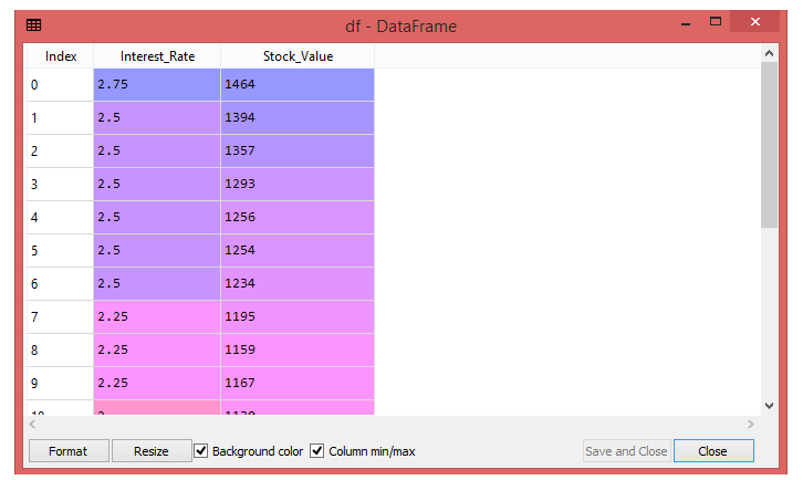
Here there are two variables Interest_Rate e (Independent variable) and Stock_Value (dependent variable). The first step is to create a Dataset by adding values to these variables.

You can see the dataset in your Spyder IDE screen by clicking on the variable explorer option.

The next step is to extract the dependent (Y) and independent (X) variables from the given dataset. The independent variable is Interest_Rate, and the dependent variable is Stock_Value.

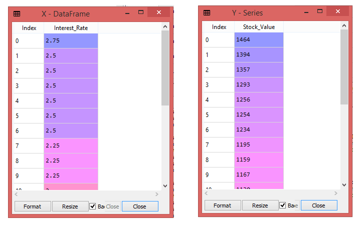
In the above image, you can see the X (Interest_Rate) variable and Y (Stock_Value) variable has been extracted from the given dataset.

Split your dataset to train and test

The train-test split is indeed a technique used to assess the performance of a machine learning algorithm. It involves dividing the dataset into two subsets: the training set and the test set. The training set is used to train the model, while the test set is used to evaluate the model's performance by measuring how well it generalizes to unseen data. This technique helps in determining how effective the algorithm is at making predictions on new data, ensuring that the model does not overfit or underfit the training data.

1. Train Set: Used to fit the machine learning model.
2. Test Set: Used to evaluate the fit machine learning model.

So, the next step is to split both variables into the Test Set and Train Set. Here, split the variables into 30:70 , this means that 30% for test set and 70% for train set.

Now, your dataset is well prepared to work on it and start building a Simple Linear Regression model for the given problem.

Fitting the data to the Training Set

In this step, fit your model to the training dataset.

Above code create an object of the class named as a "rg" and used a fit() method to fit you Simple Linear Regression object to the training set. The fit() function, train the dataset for the dependent (y_train) and an independent (x_train) variable. So that the model can easily learn the correlations between the predictor and target variables.

Prediction of test set result

Now your model is ready to predict the output for the new observations. Next, you have to provide the test dataset (new observations) to the model to check whether it can predict the correct output or not. So, you need to create a prediction vector y_pred , and x_pred , which will contain predictions of test dataset, and prediction of training set respectively.

Above code create two variables named y_pred and x_pred will generate in the variable explorer options that contain Stock Value predictions for the training set and test set.

Final Result

You can verify the result by clicking on the variable explorer option in the Spyder IDE , and also compare the result by comparing values from y_pred and y_test . By comparing these values(y_pred, x_pred), you can check how good you model is performing.

Visualizing the Train set results

The scatter () function of pyplot library will create a scatter plot of observations. In the x-axis, plot the Interest_Rate and on the y-axis, Stock_Value.

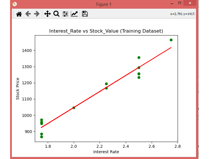
Here you can see the observations in green dots and predicted values are covered by the red regression line . The regression line shows a correlation between the dependent and independent variable.

Visualizing the Test set results

In the above section you visualized the performance of you model on the training set . The next section is the same for the Test set. The only difference from above plot is that here use the x_test , and y_test instead of x_train and y_train.

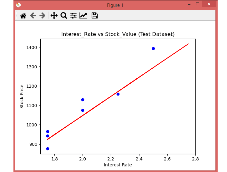
Here you can see the observations given by the blue color, and prediction is given by the red regression line . Also, you can see most of the observations are close to the regression line, hence you can confirm your Simple Linear Regression is a good model and able to make good predictions.

Full Source | Python

Conclusion

Simple Linear Regression is a fundamental machine learning algorithm used for predicting a continuous output variable based on a single input variable. It assumes a linear relationship between the input and output variables, represented by a straight line, making it a straightforward and widely used predictive modeling technique for single-variable scenarios.