Support Vector Machine Classifier | python
Support Vector Machine (SVM) is a powerful supervised machine learning algorithm that can be used for both classification and regression tasks. It aims to find the optimal hyperplane in an N-dimensional feature space that best separates the data points belonging to different classes. SVM is particularly effective in handling complex datasets and is widely used in various applications for its ability to achieve high accuracy and robustness in classification and regression tasks.
Support Vectors
- Support Vectors: These are the data points that are closest to the hyperplane and play a crucial role in defining the decision boundary. SVM focuses on these support vectors to make accurate predictions.
- Hyperplane: The hyperplane is the decision plane or surface that separates the data points belonging to different classes. In a two-dimensional feature space, the hyperplane is a line, and in higher dimensions, it is a plane or a hypersurface.
- Margin: The margin is the gap between the two parallel lines (also called hyperplanes) that are drawn on the support vectors of different classes. SVM aims to maximize this margin to achieve a better generalization and robustness in its predictions.
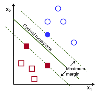
The main idea behind Support Vector Machine (SVM) algorithms is to find the decision boundary (hyperplane) that maximizes the margin between the classes. The margin is the distance between the decision boundary and the closest data points from each class, which are the support vectors. SVM focuses on correctly classifying these critical support vectors first and then aims to maximize the margin around them.
In situations where the data is not linearly separable in the original feature space, SVM can use a technique called the kernel trick to project the data into a higher-dimensional space where it becomes separable by a hyperplane. This allows SVM to handle complex and nonlinear decision boundaries effectively.
Support Vector Machines (Kernels)
SVM is a versatile algorithm that can handle both binary and multi-class classification tasks using various kernel functions. The use of more complex kernels, such as polynomial and radial basis function (RBF) kernels, allows SVM to create decision surfaces that are curved or more complex, leading to more accurate classifiers.
Plotting the decision surface for different SVM classifiers with different kernels is a useful way to visualize how they separate the data points in a dataset and can provide insights into the behavior of the classifiers in various scenarios.
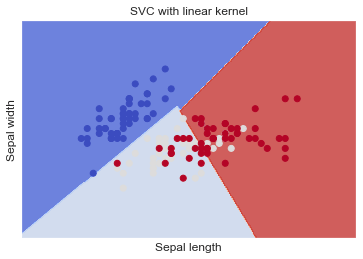
SVC with linear kernel
The implementation of SVM in scikit-learn is based on the popular LIBSVM library. While SVM is a powerful algorithm, it has some limitations in terms of scalability and multiclass support.
The fit time complexity of SVM is more than quadratic with the number of samples, which means that it can become computationally expensive for large datasets with more than a few thousand samples. As the number of samples increases, the training time can become impractical.
Additionally, scikit-learn's SVM implementation handles multiclass classification using a one-vs-one scheme, where it trains a binary classifier for each pair of classes and then combines the results to make multiclass predictions. While this approach is effective, it can be computationally expensive when dealing with a large number of classes.
Due to these limitations, SVM may not be the best choice for very large datasets or problems with a large number of classes. In such cases, other machine learning algorithms that can scale better, such as gradient boosting or deep learning models, may be more suitable.
However, SVM remains a valuable and widely used algorithm for medium-sized datasets and binary/multiclass problems with a manageable number of classes, where its strong performance and ability to handle complex decision boundaries make it an excellent choice.
Importing Libraries
Importing the Dataset (Iris data)
It is a dataset that measures sepal-length , sepal-width , petal-length , and petal-width of three different types of iris flowers: Iris setosa, Iris virginica, and Iris versicolor. The following is an example for creating an SVM classifier by using kernels.
Importing dataset
The Python Pandas module allows you to read csv files (read_csv()) and return a DataFrame object. The file is meant for testing purposes only, you can download it here: iris-data.csv .
Extracted the dependent(Y) and independent variable(X) from the dataset. Here, only consider the first 2 features of this dataset as independent variable.
- Sepal length
- Sepal width
Next step is to plot the SVM boundaries with original data as follows:
Here, you have to provide the value of regularization parameter.
SVM classifier object - linear
Create a Support Vector Classifier object by passing argument kernel as the linear kernel in SVC() function.
 Full Source - Python
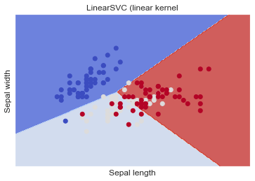
LinearSVC (linear kernel)
Similar to SVC with parameter kernel='linear' , but implemented in terms of liblinear rather than libsvm, so it has more flexibility in the choice of penalties and loss functions and should scale better to large numbers of samples.
 Full Source | Python
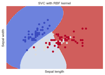
SVC with RBF kernel
When the dataset is non-linear or not separable by a simple straight line or plane, using kernel functions, such as the Radial Basis Function (RBF) kernel, is recommended in SVM.
The RBF kernel is one of the most commonly used kernel functions in SVM for handling non-linear data. It allows the SVM to map the original feature space into a higher-dimensional space where the data may become linearly separable. This transformation allows the SVM to create non-linear decision boundaries that can better fit the data and improve classification accuracy.
The RBF kernel is defined as:
where x and xi are data points, x - xi^2 is the squared Euclidean distance between the two data points, and gamma is a hyperparameter that controls the "width" of the kernel.
By adjusting the value of gamma, you can control the trade-off between overfitting and underfitting. A small gamma value makes the decision boundary smoother and may result in underfitting, while a large gamma value makes the boundary more complex and may result in overfitting.
 Full Source | Python
SVC with polynomial (degree 3) kernel
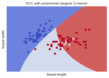 Full Source | Python
Conclusion
Support Vector Machine (SVM) Classifier is a powerful supervised machine learning algorithm used for both classification and regression tasks. It aims to find the optimal hyperplane that best separates different classes in the data by maximizing the margin between them. SVM is particularly effective in handling non-linear data by using kernel functions to map the data into higher-dimensional spaces where it becomes separable.